Abstract
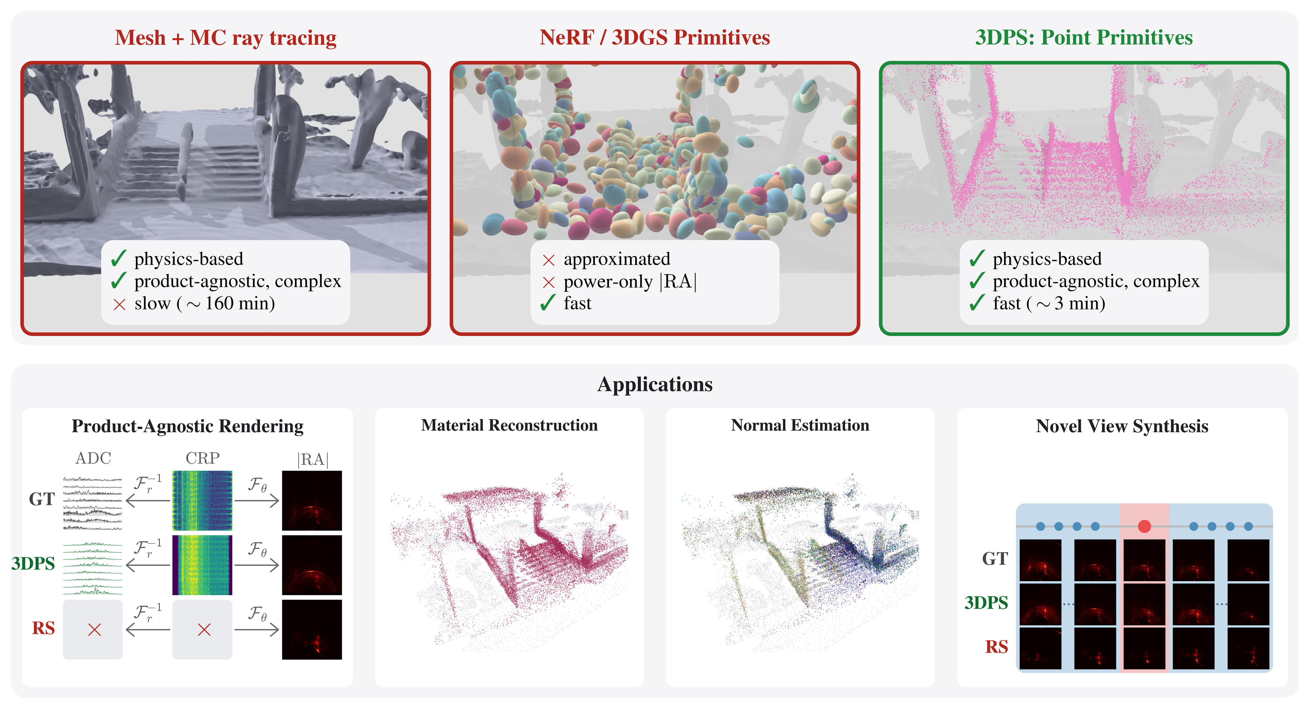
Solving novel view synthesis (NVS) for millimeter-wave (mmWave) radar requires a renderer that is multi-viewpoint-tractable, physically faithful, and complex-valued. No prior method achieves these three properties simultaneously. Physically based radar renderers must condition radar synthesis not only on sensor pose, but also on the full antenna array geometry, waveform configuration, and beam patterns. Differentiable Monte Carlo (MC) ray tracers implement the radar forward model directly with explicit material modeling and complex outputs, but do not scale to the multi-view optimization NVS demands. Optical-NVS ports of NeRF, hash grids, and 3D Gaussians train fast but discard phase and replace explicit material modeling with opaque learned features, restricting them to power-only range–azimuth (RA) magnitudes. We propose 3D Point Splatting (3DPS), the first differentiable point renderer for radar, derived directly from the standard solid-angle form of the radar equation. Each oriented 3D point carries an ITU-R P.2040 material model, evaluated in closed form, with the resulting complex phasor splatted into range bins through a precomputed point spread function (PSF). Complex-valued output makes the renderer product-agnostic: the same optimized scene yields ADC, complex range profile (CRP), and RA outputs through standard FFT pipelines without retraining for each format. On six outdoor ColoRadar scenes, 3DPS reaches 0.587 mean Pearson correlation on held-out RA images, 1.8–7.2× over RadarSplat, Radar Fields, and DART. Training takes ∼3 minutes per scene on a single RTX 4090, ∼50× faster than the SOTA MC ray tracer’s projected per-scene cost.
Method Overview
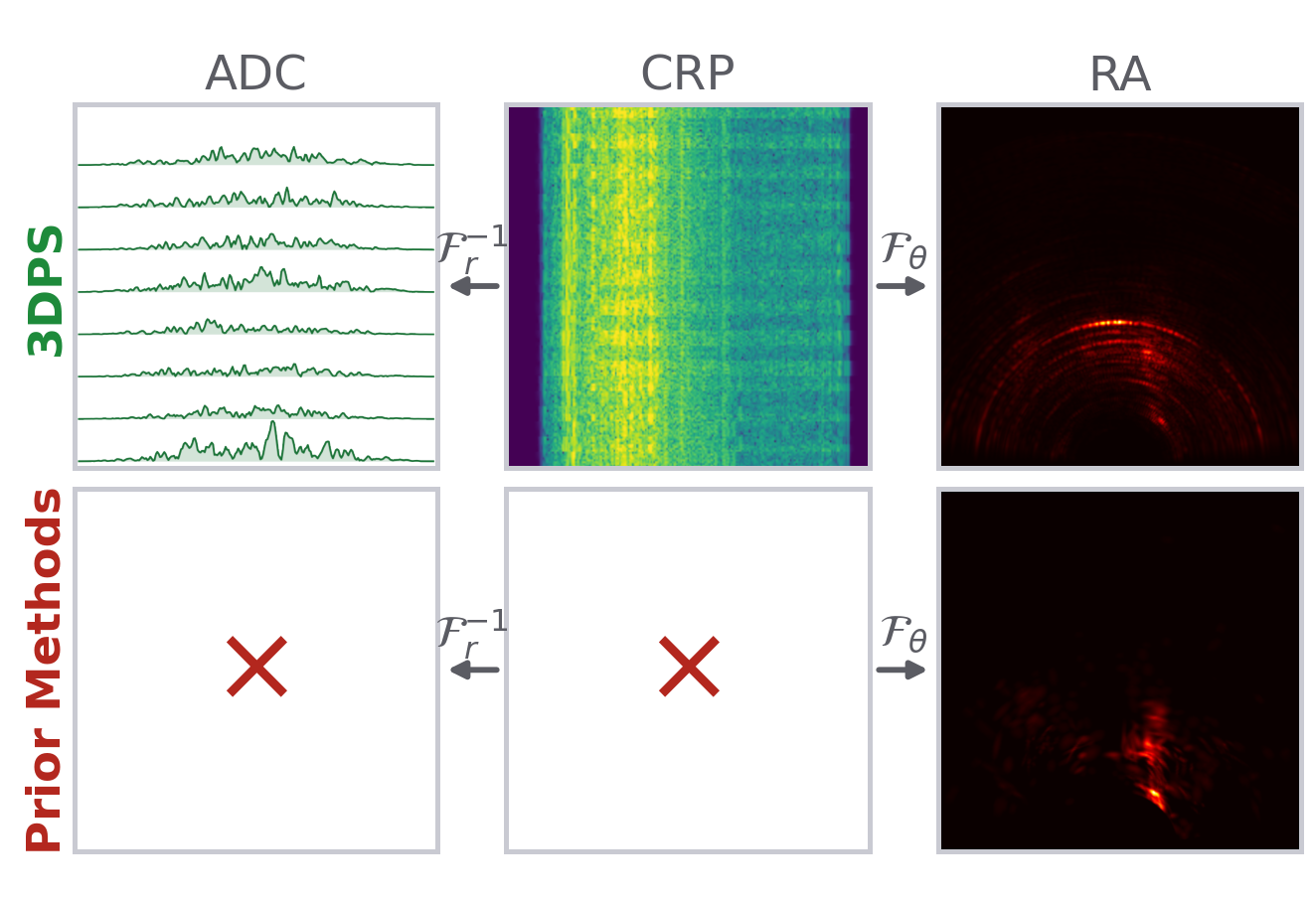
3DPS optimizes point primitives, the optimal design choice prescribed by the solid-angle radar rendering equation. Each carries position, normal, and ITU-R P.2040 material parameters, and is initialized from LiDAR. The forward model splats each point’s complex phasor into its range bins through a precomputed 15-tap Hann-window point spread function, by evaluating antenna gain, the BSDF, and the geometric phase for each (TX, RX) pair in closed form. The result is a complex range profile, and standard FFTs make both the raw ADC and range–azimuth map accessible. Gradients from a range–azimuth loss flow back to every point’s normal and material parameters.

3DPS fits oriented points (positions, normals, and materials) by splatting them directly into the measured complex range profile, one invertible transform away from raw ADC. A joint eight-viewpoint fit runs in 3.17 min/scene against 77.59 for mmIR on a RTX 4090 GPU.
Ray Tracing vs Splatting
Ray tracing methods require LiDAR meshing, tracing for hit points, raw ADC samples per (TX, RX) pair per hit, and a range-profile transform. 3DPS keeps LiDAR points as scattering sites (no meshing or tracing) and splats these points onto the complex range profile directly (fewer scatter-adds). 3DPS fits eight viewpoints in 3.17 min against 77.59 for mmIR on an RTX 4090 GPU.
Training
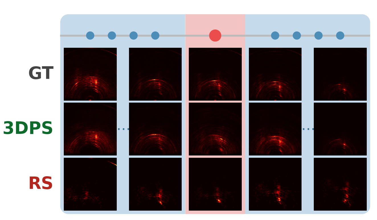
We train on six outdoor ColoRadar scenes, each with nine consecutive cascaded-radar poses along a real trajectory: eight poses are fitted jointly against one shared scene and the middle pose is held out entirely. The real raw capture at every training pose is the only supervision. Below, all eight views converge together over 500 iterations, mean |RA| correlation climbing from 0.226 to 0.842, with the four adaptive-density rounds visible as dips.
The eight training views of one scene, each measured map against 3DPS’s render of it, as the joint fit converges. One scene is optimized against all eight at once; the held-out ninth pose is never shown to the fit and is reported in the results below.
3DPS Fits Explicit Scene and Sensor Representations
Each point stores a position, a surface normal and an ITU-R P.2040 material. Each viewpoint stores the radar's full array geometry and pose. Because the parameters are physical, one fitted scene re-renders to raw ADC, complex range profile or range–azimuth through the standard transforms, with no retraining per format. Note that the middle pose of every trajectory is withheld from fitting, so the maps shown there are a prediction rather than a reconstruction.
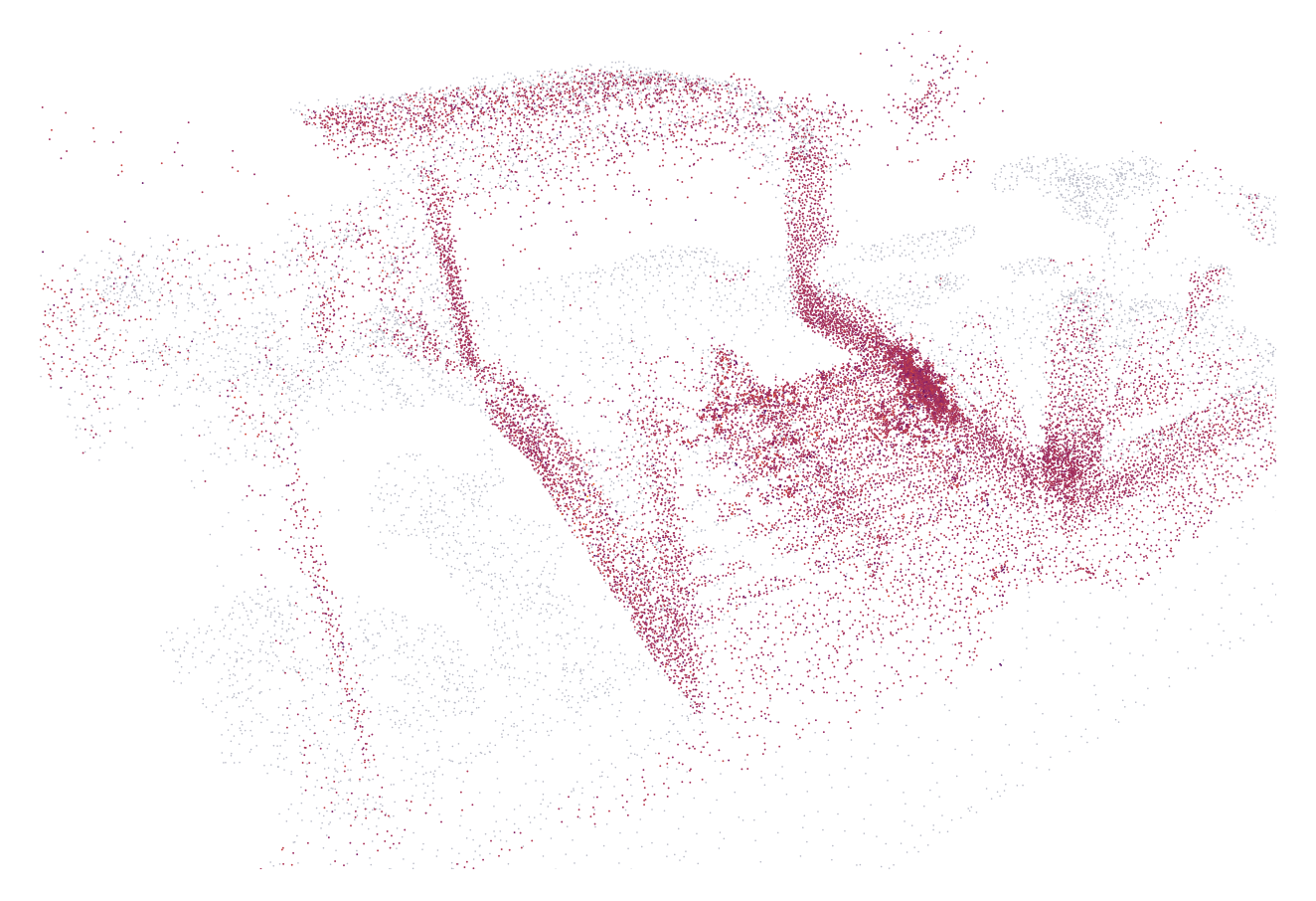
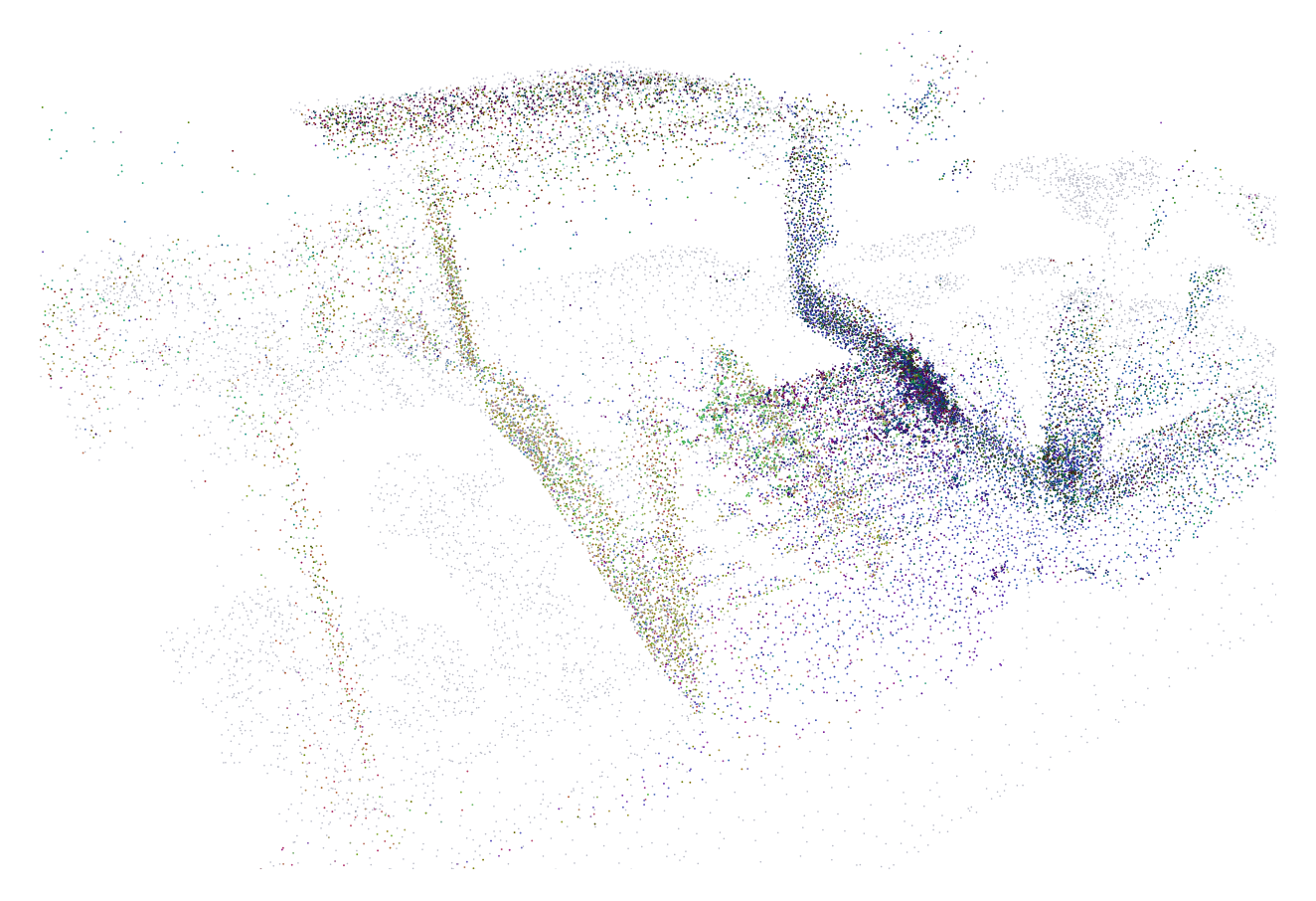
Each scene contains 20,000 oriented points, shown in grey by default or coloured by the fitted normal or the fitted relative permittivity ε′r, against the translucent LiDAR mesh they were initialized from. Blue spheres are the fitted poses and the red one is withheld, each with a boresight arrow and a 67.8° × 19.8° field of view. Selecting a pose shows its measured and rendered range–azimuth maps and their |RA| correlation.
Results: Sparse Novel View Synthesis
On the held-out view, 3DPS reaches 0.587 mean RA correlation across the six outdoor scenes. The optical-NVS ports either lose all the energy or collapse it into a few lobes, while 3DPS reconstructs the dominant scatterers and resolves them along range and azimuth. mmIR, the SOTA ray tracing baseline, reaches 0.454. 3DPS is 1.3× more accurate on NVS, and about 24× faster.

The held-out view of each of the six ColoRadar scenes, identical normalization across every panel; the per-cell number is |RA| Pearson correlation against the measured frame. 3DPS keeps the arcs where the ground truth has them, at roughly the right strengths.